2D Neural Field Implementation
For the first part of the project, I implemented a simplified 2D version of a neural field. This required learning a continuous representation of a 2D image through a neural network that maps pixel coordinates to RGB values.
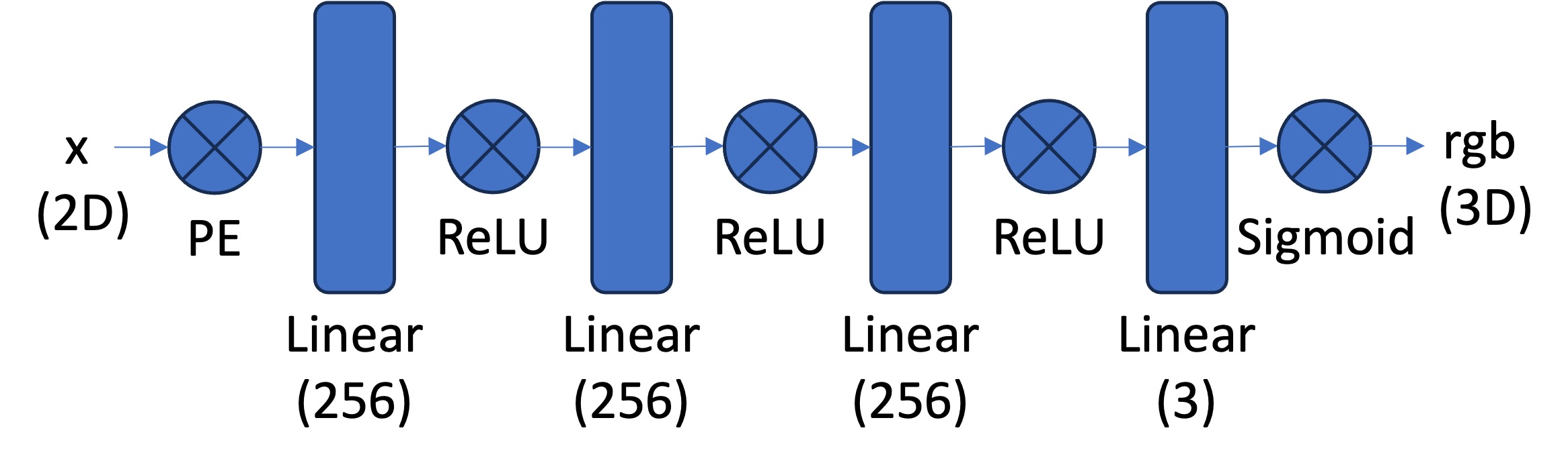
The network architecture consists of a multi-layer perceptron (MLP) with positional encoding of the input coordinates. I implemented positional encoding with $L=10$ frequency bands, transforming the 2D coordinates into a 42-dimensional vector using sinusoidal functions:
$$PE(x) = \{x, sin(2^0\pi x), cos(2^0\pi x), sin(2^1\pi x), cos(2^1\pi x), ..., sin(2^{L-1}\pi x), cos(2^{L-1}\pi x)\}$$
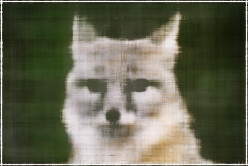
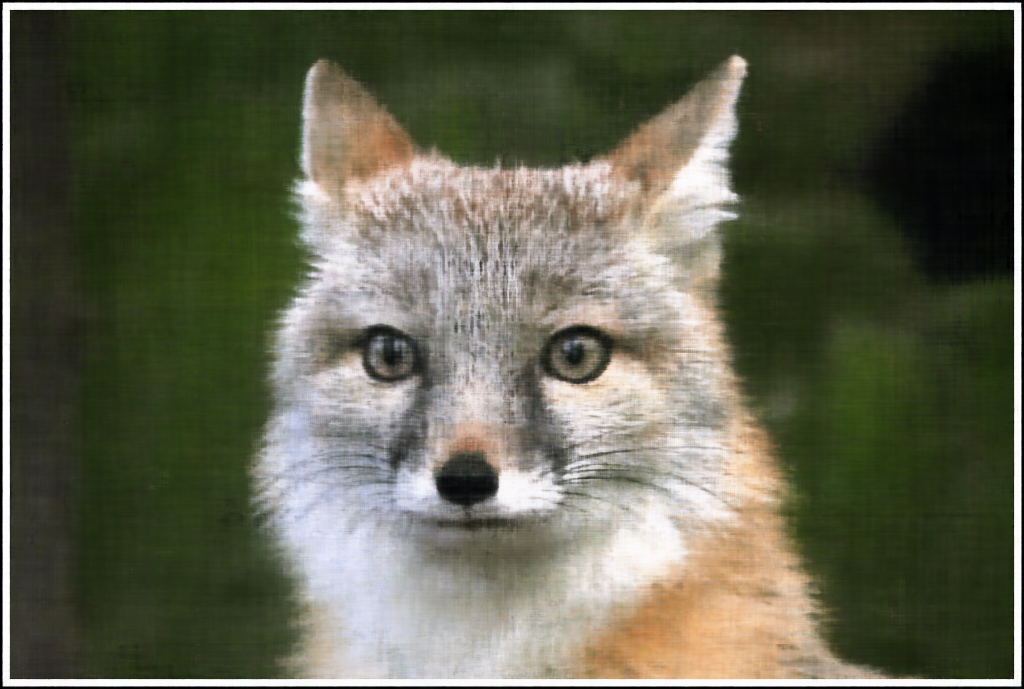
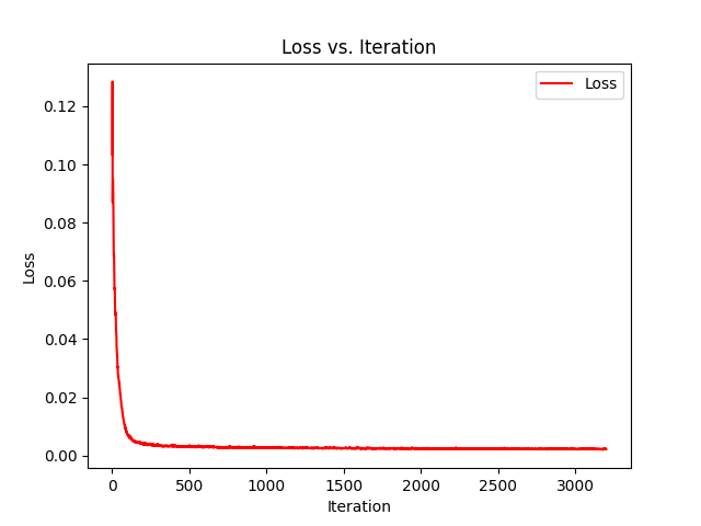
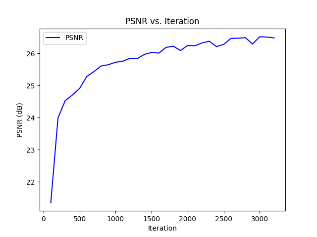
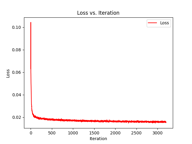
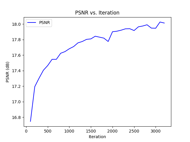
For training, I implemented a data loader that randomly samples 10,000 pixels per batch from the input image. The model was trained using MSE loss and the Adam optimizer with a learning rate of 0.01. Training for 3200 iterations achieved a PSNR of 26.7 dB on the test image. Through a little bit of experimentation, I found that increasing the network width beyond 256 didn’t really do anything and that reducing the positional encoding frequencies below $L=8$ reduced the quality of high frequency details.
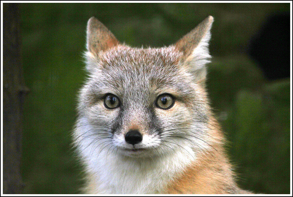
Original Fox Image
100 Iterations
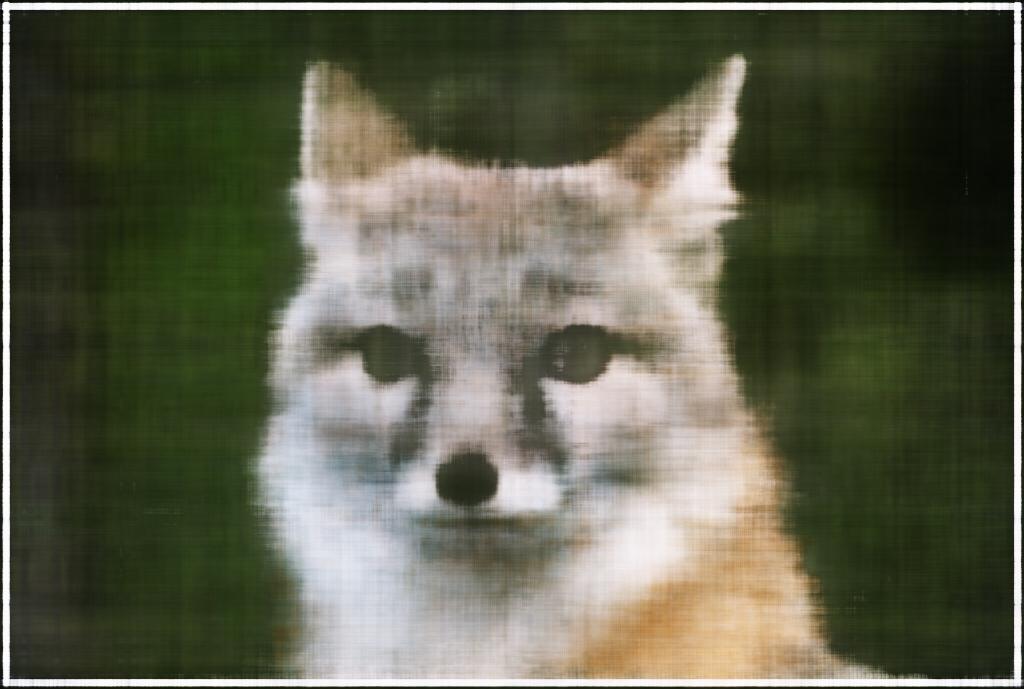
200 Iterations
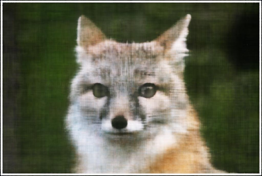
400 Iterations
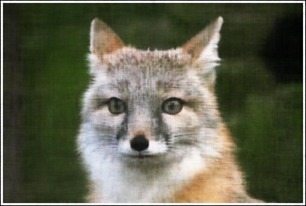
800 Iterations
1600 Iterations
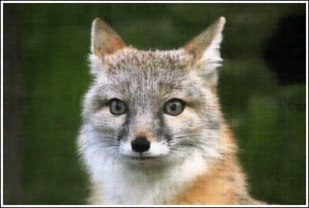
3200 Iterations
Original
Learned
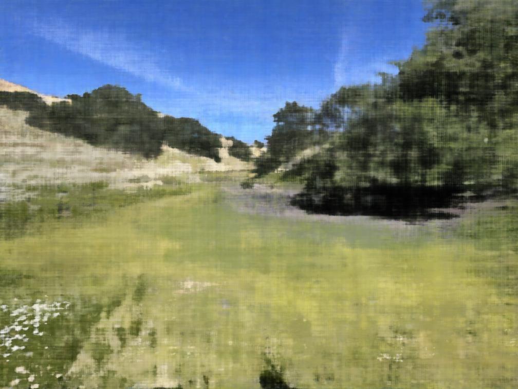
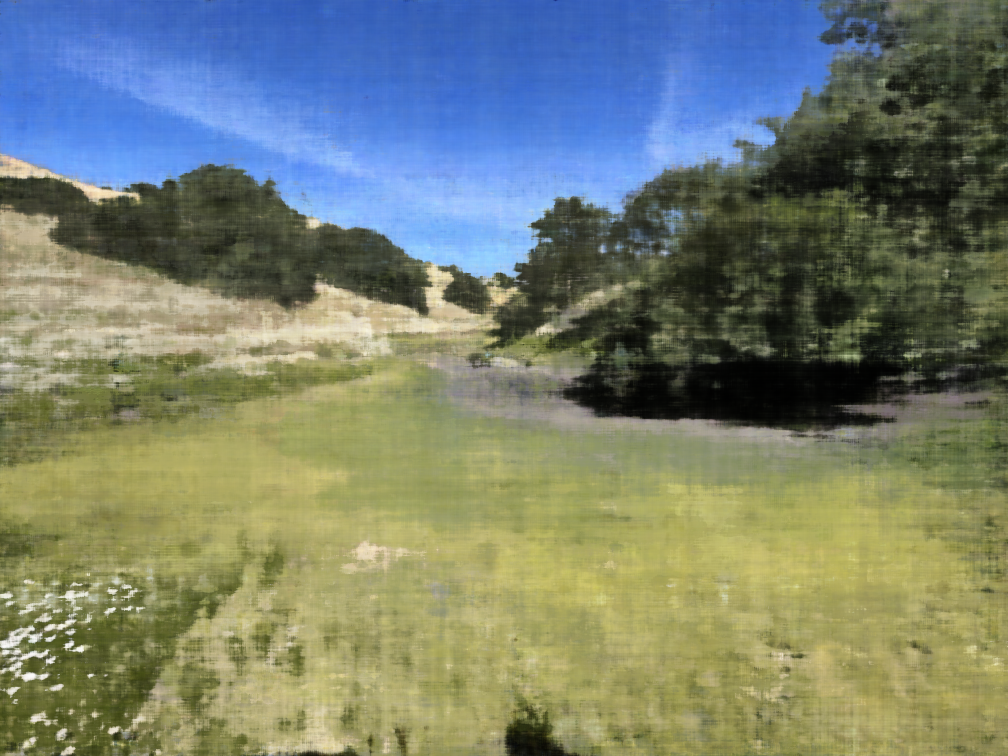
Trying another image, notably one with more high frequency data, and had a lower PSNR.
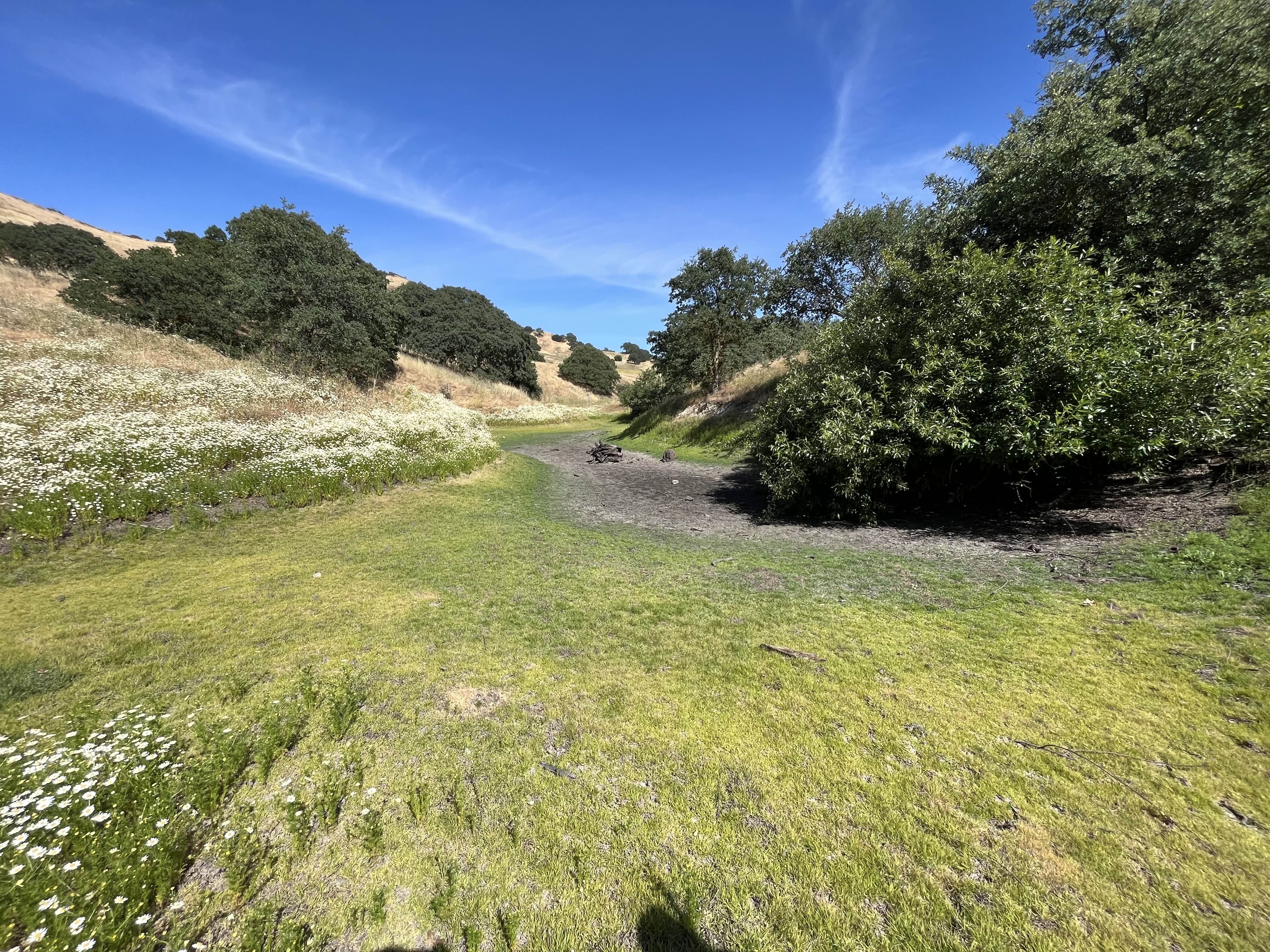
Original Fossil Hill Trail Image
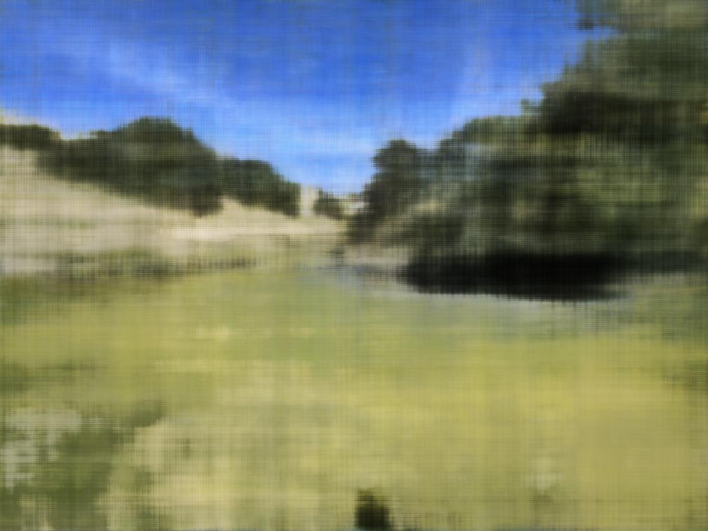
100 Iterations
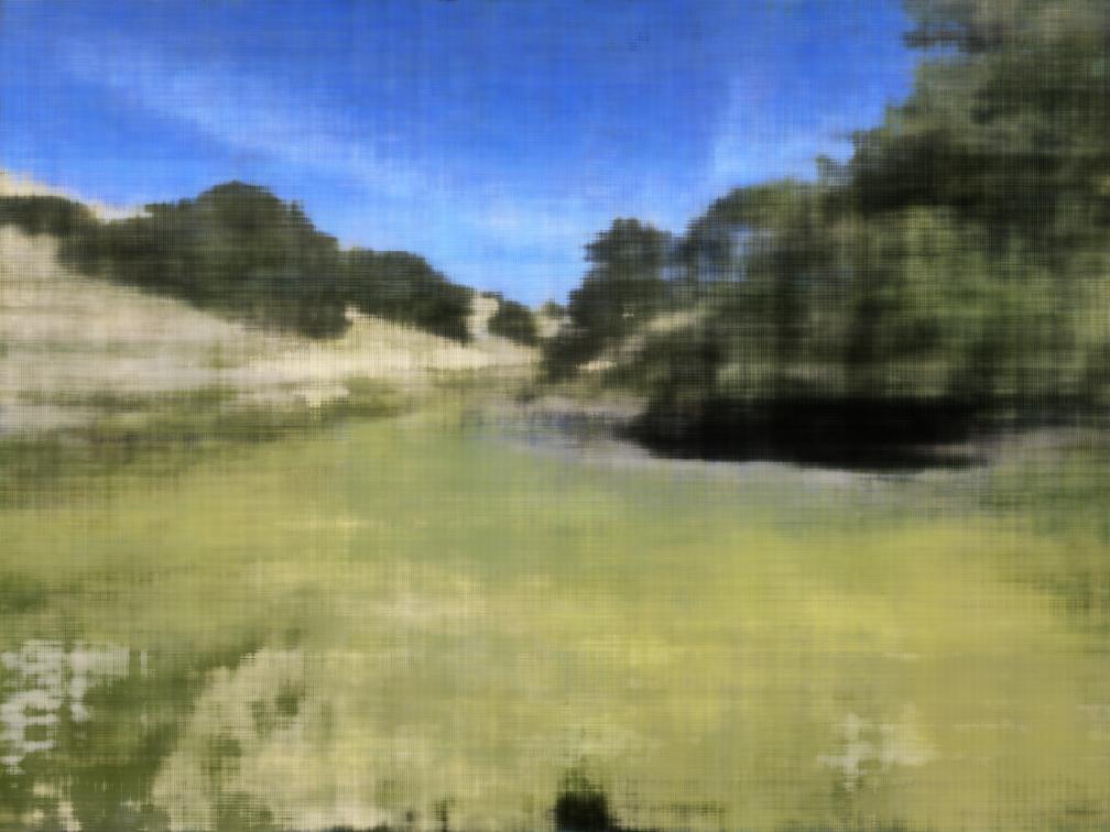
200 Iterations
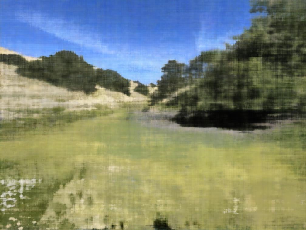
400 Iterations
800 Iterations
1600 Iterations
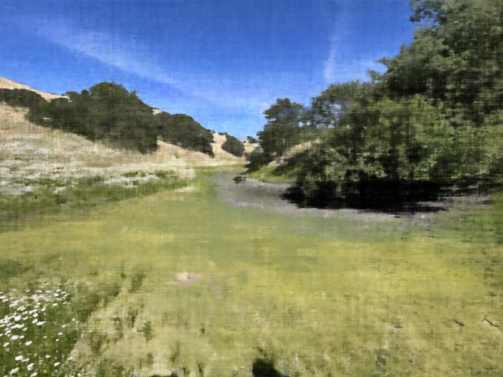
3200 Iterations
Original
Learned
Fit a Neural Radiance Field from Multi-view Images
Create Rays from Cameras
The first thing I had to do was to define some transformations from pixel coordinates to world-space rays.
First is a camera-to-world transformation. The function transform(c2w, x_c) converts points from camera space to world space using homogeneous coordinates.
Next is a pixel-to-camera conversion. The function pixel_to_camera(K, uv, s) inverts the projection process, transforming pixel coordinates back to camera space. Given pixel coordinates (u, v), depth s, and the camera intrinsic matrix K, it reconstructs the 3D point in camera space.
Finally, ray generation. The function pixel_to_ray(K, c2w, uv) combines the previous two transformations to generate rays for each pixel.
Sampling Implementation
The sampling part of the NeRF implementation involves two key components: sampling rays from images and sampling points along those rays. This is the means by which the neural network learns.
To samples rays from images, I made a function to sample rays across multiple images by treating all image pixels as a single pool. This approach involves flattening the pixels and randomly selecting rays in one step. To do this, I made a RaysData class with a sample_rays function which takes as input and outputs sampled rays. I had to adjust the UV coordinates by adding 0.5 to center them within each pixel, but these adjusted coordinates were then converted to ray origins (rays_o) and directions (rays_d) using camera intrinsics and extrinsics.
To sample points along each ray, I made a sample_points_along_rays function. It starts by generating evenly spaced samples along the ray using np.linspace, then when a perturb flag is set to true, a random offset is added to the sample positions to introduce variation during training.
Putting it all together
To validate all the previous work, we visualize the results:
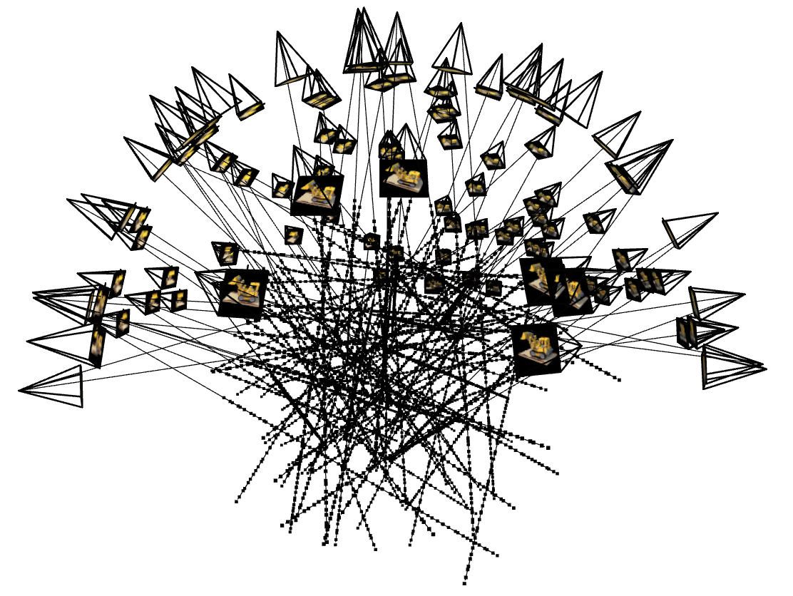
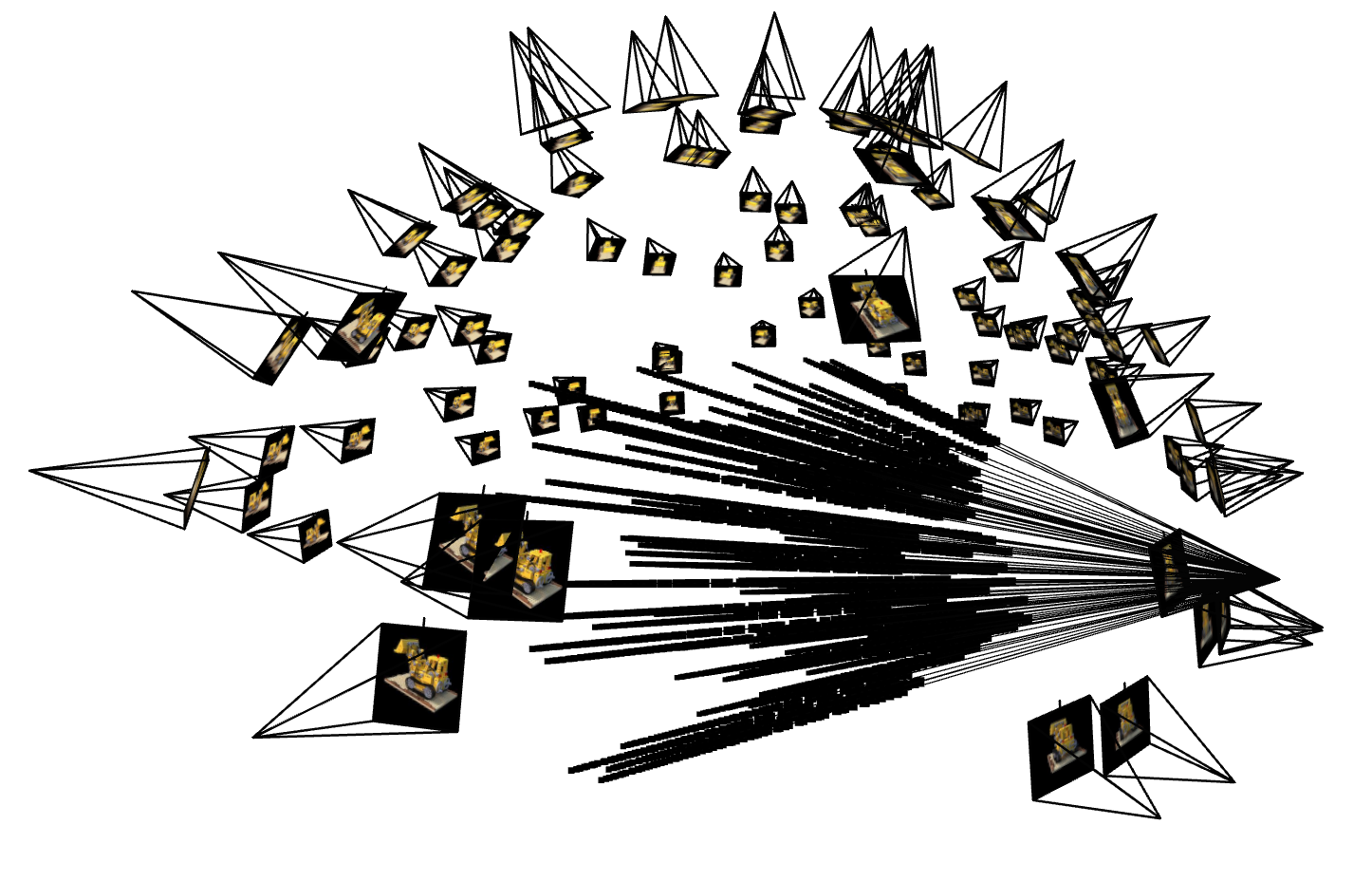
We can see that we are correctly construction rays from the cameras and that the points are correctly sampled along the rays. Thus the network is able to learn the correct density and color of the points, which we'll describe next.
Neural Radiance Field
The network is designed to predict the density and color of points in space.
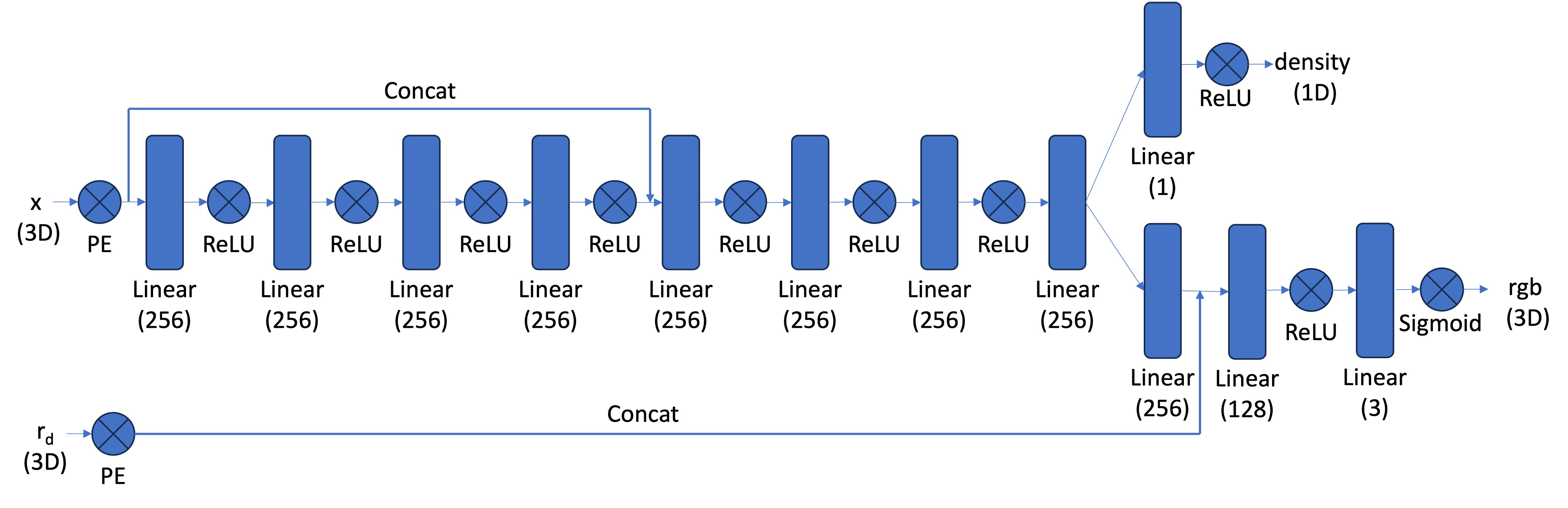
We positionally encode the positions and ray directions using $L=10$ and $L=4$ frequencies, respectively. For color prediction, the intermediate features are processed further, concatenated with the encoded ray directions, and then passed through additional layers to predict RGB values. We apply a sigmoid activation to ensure the RGB output is between 0 and 1. This architecture also includes skip connections to preserve the input signal and effectively model the view-dependent and geometric characteristics of the 3D scene.
Volume Rendering
Volume rendering is how we synthesis novel views in NeRFs. The color of a ray \( C(\mathbf{r}) \) is determined by integrating the contributions of points along its path, writen as: \begin{align} C(\mathbf{r}) = \int_{t_n}^{t_f} T(t) \sigma(\mathbf{r}(t)) \mathbf{c}(\mathbf{r}(t), \mathbf{d}) \, dt, \quad T(t) = \exp \left(-\int_{t_n}^t \sigma(\mathbf{r}(s)) \, ds\right), \end{align} where \( \sigma(\mathbf{r}(t)) \) represents the density at a point \( \mathbf{r}(t) \), \( \mathbf{c}(\mathbf{r}(t), \mathbf{d}) \) is its emitted color, and \( T(t) \) is the transmittance, capturing the fraction of light that reaches \( t \) without being absorbed.
In the discrete case, this is approximated by: \begin{align} \hat{C}(\mathbf{r}) = \sum_{i=1}^N T_i \left(1 - \exp(-\sigma_i \delta_i)\right) \mathbf{c}_i, \quad T_i = \exp\left(-\sum_{j=1}^{i-1} \sigma_j \delta_j\right), \end{align} where \( \delta_i \) is the distance between consecutive samples, and \( T_i \) is the accumulated transmittance up to the \( i \)-th point. This formulation is differentiable which means we can train the network to predict densities \( \sigma_i \) and colors \( \mathbf{c}_i \), allowing for our pretty novel view synthesis.
To implement this and calculate these integrals, we get the transmittance and alpha values for each sampled point along a ray to weight how much it contributions to the color to the final image.
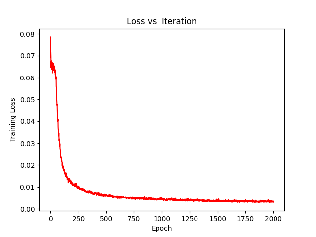
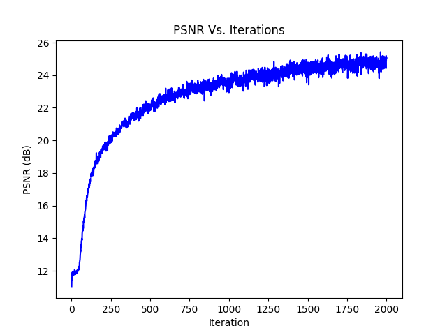
Training
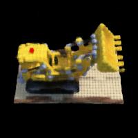
After 2000 iterations with learning rate of 0.0005 and a batch size of 10,000 rays, we get the following results:
~0 Iterations
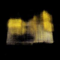
~100 Iterations
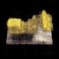
~200 Iterations
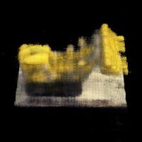
~400 Iterations
~800 Iterations
~1600 Iterations
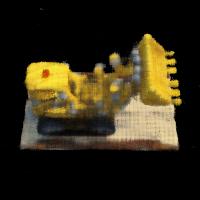
Results
After everything is all said and done, we can stitch together novel views of our scene and see that our neural representation does a pretty decent job.