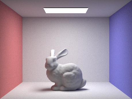
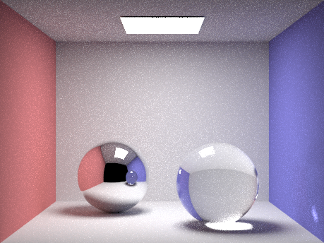
Introduction
My last major project, Rodent-Ray-Tracer, was my first ever ray tracer and introduction into path tracing, physically based rendering, optics, probability, and so much more. The project was an entirely self led initiative where I had to teach myself a plethora of intimidating mathematics, physics, and computer science topics. Since it was the very definition of a passion project, the goals and means to get them were arbitrary- it was heaps and bounds of fun, but not the most rigorous in its execution. Since then I’ve been able to take Berkeley’s CS 184, Computer Graphics and Imaging, and receive some absolutely incredible lectures on the precise topics that I had come across and maybe even implemented but yet to fully understand in a formal context: radiometry, monte carlo integration, importance sampling, acceleration structures, and more. This project is the formalization of my understanding of these essential concepts.
Problem Statement
Creating photorealistic images involves accurately simulating how light interacts with objects in a scene. Traditional rendering methods often struggle with the computational complexity and inefficiencies associated with realistic light transport. Path tracing, while more accurate, requires significant computational power and time, especially when dealing with complex scenes. The main challenges include efficiently simulating light paths, managing the vast number of possible interactions between light and surfaces, and ensuring that the rendering process is both accurate and feasible within a reasonable timeframe. This project addresses these challenges by implementing advanced techniques such as backward ray tracing, efficient intersection algorithms, and the use of acceleration structures like Bounding Volume Hierarchies (BVH) to significantly enhance rendering performance without compromising on quality.
Technical Approach
Mathematics of Ray Tracing
Fundamentally, path tracing is about simulating the path of light as it travels from a source into our sensor, be it our eyes or camera, and recording the light/photons into a matrix or grid of intensity/color cells. The most naive way to do this is to simulate the path of every photon from a source of light. This is naive because there are going to be a lot of photons emitted from any given light source which don't make their way into our eyes. So rather than running a simulation on photons which fly off into space and are never seen, let's only focus on simulating the light which makes it into our eyes. But how do we determine which photons emit from a light source and make their way into our eyes without simulating every light source to find out? He solution: backwards ray tracing. Backwards ray tracing is the process of sending rays out from our eyes, effectively backwards photons, into a scene and seeing whether what they hit is indeed a light source or not. Because ray tracing follows the model of geometric optics which assumes euclidean space, meaning light travels in straight lines, then if a straight line can be drawn from our eyes to the surface of an emissive surface, then we should see light from it directly. Another problem is that there is, for our intents and purposes, an infinite amount of photons landing.
Ray-Sphere Intersection
The first thing you do with ray tracing is ofcourse raytrace a sphere. But how do you check if and where a ray intersects with a sphere? Well, this gets reduced to solving a quadratic equation.
Ray-Triangle Intersection
Another, more practical way of representing an object's surface is with triangles. That is because every surface in the real world which is continuous is locally manifold or flat at every point. Thus given an infinite number of flat 2D shapes, we could compose them to represent any surface we want. However, since computers do not have infinite resources in our finite world, we must discretize and approximate things. We use triangles because they are the simplest polygon and can be used to compose all other polygons. Thus the surface geometry of any 2D or 3D object can be modeled with triangles
Our problem is still figuring out how to algorithmically check if light ever hits the surface of an object. Since we assume light travels in a straight line, and every object in our scene is composed of triangle primitives, another way to state our problem is to find out how to check if our light (line) ever intersects with our scene geometry (triangles). To put it simply, we need an algorithm for checking ray-triangle intersections. Fortunately this can be boiled down even more because we assume every triangle is flat and thus is just an area in a plane. Using math we learned in analysis geometry/multivariable calculus and barycentric coordinates, we know how to algebraically check whether and where a line intersects a plane and if a point (the line-plane intersection point) lies within the area.
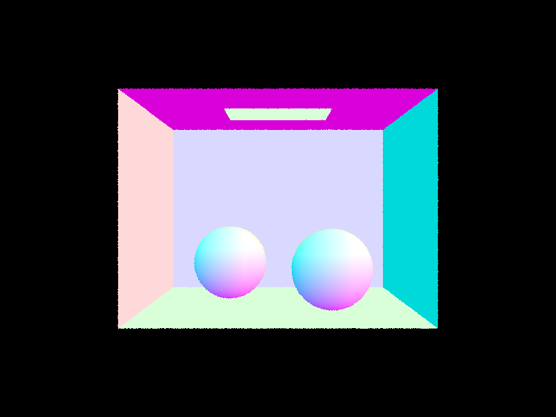
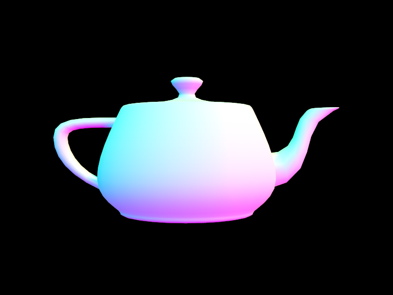
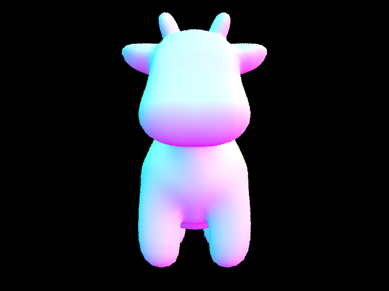
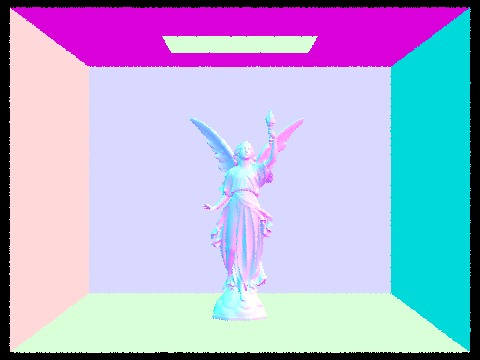
Implementing ray-sphere and ray-triangle intersections, we're able to render these simple scenes with normal shading:
Fortunately again, this problem of ray-triangle intersection is so fundamental to raytracing, some very efficient algorithms have been devised by some very smart people in the past to make this as fast as possible. As one can imagine, if we want to render an NxM image and our scene objects have P primitives, in the best case, we’re going to be running an intersection algorithm NxM times and at worst NxMxP times.
Let N, M, P = 1000, giving us a spantty standard resolution and an embarrassingly low polygon count for a scene. This is 1000^3 = (10^3)^3 = 10^9 = 1,000,000,000. One billion of any operation on any machine is going to take some time. However, in 2019, Pixar boasted having scenes with polygon counts in the trillions, so what gives? How are these scenes being rendered in our lifetimes given the algorithmic time complexity we see at hand.
Data Structures and Algorithms in Ray Tracing
Scene Representation
Imagine a typical scene, such as a living room filled with furniture, decorations, and perhaps a teapot on a table. This scene consists of numerous geometric primitives that define each object within it. When rendering the scene, rays are cast from the camera into the space to determine visibility and light interaction for each pixel on the screen. In a naive approach, every ray would need to be tested against every primitive to check for intersections. While this method is accurate, it is highly inefficient and impractical, especially in complex scenes where most rays interact with only a few objects and miss the majority.
Consider our scene again. The teapot occupies only a small fraction of the entire space, meaning that many rays will pass through empty areas without intersecting the teapot or other objects. Without optimization, the ray tracer would waste valuable time checking for intersections in these empty spaces. Since our scenes and objects are composed of geometric primitives, there’s no inherent order to these primitives. But let’s see if there's a way we can define some structure on our data (see what I did there? ;)) and exploit it to improve the efficiency of the ray tracing process.
Acceleration Structures
Achieving accurate rendering is crucial, but doing so efficiently—within our lifetimes—is equally important. The enormous amount of computations and data involved in path tracing necessitates the use of specialized data structures and algorithms to manage the process effectively. This is where acceleration structures come into play.
Acceleration structures are designed specifically to address inefficiencies like those seen with our teapot example. By organizing geometric data in a way that enables efficient access and exclusion of irrelevant parts of the scene, these structures drastically reduce the number of intersection tests required during rendering.
- Bounding Volume Hierarchies (BVH): In this method, the scene is divided into a hierarchy of nested bounding volumes, each encapsulating a group of primitives. When a ray is cast, it is first tested against these bounding volumes. If a ray misses a bounding volume, all the primitives it contains are immediately discarded, avoiding unnecessary computations.
- k-D Trees: This structure recursively subdivides the scene along its spatial dimensions, organizing primitives into a binary tree. Like BVH, if a ray doesn’t intersect a certain region of the k-D tree, all associated primitives are excluded from further testing.
- Grids: A uniform grid divides the scene into equally sized cells, each containing a list of primitives. Rays traverse the grid, testing for intersections only within the cells they pass through, which can be much more efficient than testing against all primitives in the scene.
These acceleration structures are not just useful—they are essential for making path tracing feasible in complex scenes. By leveraging data structures and algorithms, we not only ensure the accuracy of the rendering but also achieve this within a reasonable timeframe, making advanced rendering techniques like path tracing practical for real-world applications.
Bounding Volume Hierarchy
We construct our BVH in a very simple and balanced manor. Given a list of primitives, we compute the bounding box of all the primitives. If the number of primitives exceeds a threshold, we compute the axis of the longest side of the bounding box and sort the geometry along its position’s coordinate for that axis. Finally we split this sorted list in half, recusing until the list’s length is below the initial threshold.
The asymptotic difference between performing ray intersection with and without a BVH is the difference between O(log N) and O(N) respectively. We know for large N the clock time difference becomes astronomical. Our results show that the BVH acceleration resulted in an order of magnitude increase in performance.
Without BVH:
- Rays processed per second: 7,600
- Average intersection tests per ray: 1,073
- Time to render: 22.7296 seconds


With BVH:
- Rays processed per second: 1,546,600
- Average intersection tests per ray: 7
- Time to render: 0.1046 seconds
Show images with normal shading for a few large .dae files that you can only render with BVH acceleration.
Mathematics of Path Tracing
When rendering a scene in computer graphics, path tracing simulates the complex behavior of light by tracing the paths of photons as they interact with surfaces. The goal is to capture not just direct illumination but also how light reflects and refracts between various surfaces before reaching the observer. This involves solving the rendering equation, which integrates over all possible light paths to determine the outgoing radiance at a point.
In path tracing, the behavior of light is modeled by tracing the paths of photons as they reflect and refract through a scene. Each photon’s path is a solution to the rendering equation, which is an integral equation that computes the outgoing radiance \( L_o(x, \omega_o) \) at a point \( x \) in direction \( \omega_o \) by considering the sum of emitted and reflected light contributions:
\[ L_o(x, \omega_o) = L_e(x, \omega_o) + \int_{H^2} f_r(x, \omega_i, \omega_o) L_i(x, \omega_i) (\omega_i \cdot n) \, d\omega_i \]
Light Transport Equation
The Light Transport Equation (LTE), formalized by James Kajiya, describes how light is transferred through a scene by combining both direct and indirect illumination. It integrates the effects of light emitted by sources and the light that is reflected from other surfaces within the scene. The LTE is crucial for simulating realistic lighting, as it provides a comprehensive model of light interaction in a physical environment.
The Light Transport Equation, or rendering equation, is an integral equation describing the balance of radiance leaving a point in a particular direction. It is expressed as:
\[ L_o(x, \omega_o) = L_e(x, \omega_o) + \int_{\Omega} L_i(x, \omega_i) f_r(x, \omega_i, \omega_o) (\omega_i \cdot n) \, d\omega_i \]
Global Illumination
Global Illumination (GI) encompasses techniques that simulate how light interacts with surfaces throughout a scene, not just from direct sources. It accounts for the complex interactions of light, including reflections, refractions, and indirect illumination effects such as color bleeding and soft shadows. GI aims to produce images that closely resemble real-world lighting by capturing these intricate light interactions.
Global Illumination techniques aim to solve the full rendering equation, taking into account both direct and indirect lighting. This often involves computing the sum of an infinite series of light bounces:
\[ L_o(x, \omega_o) = L_e(x, \omega_o) + \sum_{i=1}^{\infty} \int_{\Omega_i} L_i(x_i, \omega_i) f_r(x_i, \omega_i, \omega_o) (\omega_i \cdot n_i) \, d\omega_i \]
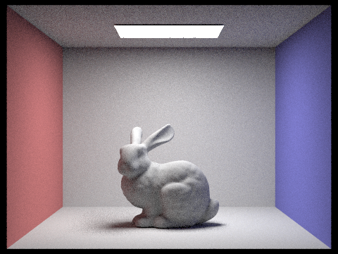
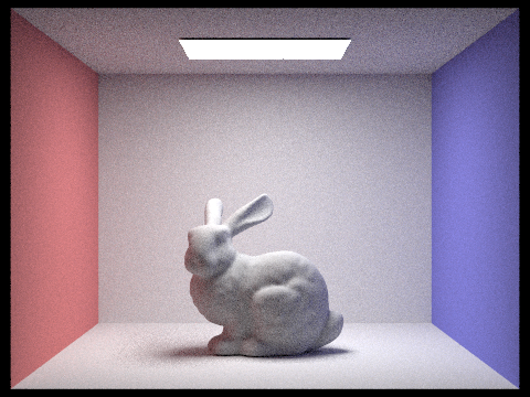
The difference between integrating increasing number of light bounces:
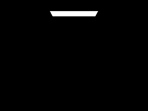
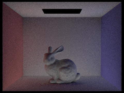
Global Illumination is made from both direct and indirect lighting:
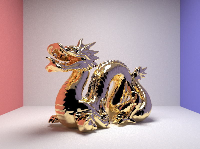
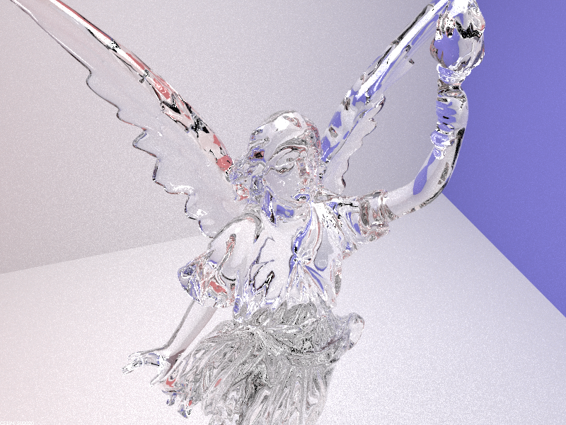
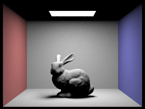
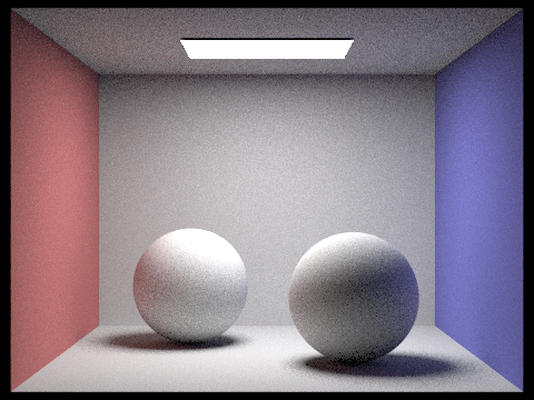
Some pretty renders with global illumination:
Monte Carlo Integration
Monte Carlo Integration is used to estimate the integral representing the light contribution at a point by averaging random samples. This statistical method is applied in path tracing to approximate the integral of light paths through a scene, improving the accuracy of rendered images with sufficient samples.
Monte Carlo Integration estimates an integral by taking the average of a function evaluated at random sample points. For the rendering equation, this is expressed as:
\[ L_o(x, \omega_o) \approx \frac{1}{N} \sum_{j=1}^{N} \left[ \frac{f_r(x, \omega_i^j, \omega_o) L_i(x, \omega_i^j) (\omega_i^j \cdot n)}{p(\omega_i^j)} \right] \]
Sampling Techniques
Efficient sampling techniques focus computational resources on significant light paths to solve the Light Transport Equation effectively. Techniques such as light sampling prioritize rays interacting with light sources, reducing variance and improving convergence in the rendered image.
Efficient sampling techniques reduce the variance in Monte Carlo estimates by focusing on important paths. For example, in importance sampling, samples are drawn according to a probability density function \( p(x) \) that is proportional to the function being integrated:
\[ \int f(x) \, dx \approx \frac{1}{N} \sum_{i=1}^{N} \left[ \frac{f(x_i)}{p(x_i)} \right] \]
Russian Roulette
Russian Roulette is a technique used to probabilistically terminate light paths to manage computational efficiency. After a certain number of bounces, each ray has a probability of being terminated, and its contribution is adjusted to ensure energy conservation in the final image.
Russian Roulette reduces computational load by terminating light paths probabilistically. If a path is terminated at a bounce with probability \( P \), the contribution of that path is scaled by \( \frac{1}{P} \) to maintain unbiasedness:
\[ \text{Contribution} = \frac{1}{P} \text{ (if terminated)} \]
Bidirectional Scattering Distribution Function (BSDF)
The Bidirectional Scattering Distribution Function (BSDF) is a fundamental concept in computer graphics that describes how light interacts with surfaces. It encompasses both reflection and transmission (refraction) models, providing a unified framework for simulating various material properties.
Path tracing relies on simulating light interactions with various surfaces to achieve realistic images. The interaction of light with a surface is described by the Bidirectional Reflectance Distribution Function (BRDF), which encapsulates different reflection and transmission properties. This overview examines three critical reflection models: Lambertian reflection, combined reflective and refractive surfaces (such as glass), and the microfacet model.
Lambertian Reflection Model
The Lambertian reflection model is used to simulate perfectly diffuse surfaces, where light scatters uniformly in all directions, independent of the viewing angle. Based on Lambert's Cosine Law, the intensity of the reflected light depends on the cosine of the angle between the incident light and the surface normal.
The reflected radiance \( L_o \) from a Lambertian surface is expressed as:
\[ L_o(x, \omega_o) = \frac{\rho}{\pi} L_i(x, \omega_i) (\omega_i \cdot n) \]where \( \rho \) represents the surface's albedo (reflectance), \( L_i(x, \omega_i) \) is the incident radiance, \( \omega_i \) is the incident light direction, and \( n \) is the surface normal.
Reflective and Refractive Models (Combined Reflection and Transmission)
Materials like glass and water exhibit both reflective and refractive properties. The interaction of light with these materials involves a combination of reflection and transmission, governed by the Fresnel equations.
Glass BSDF (Bidirectional Scattering Distribution Function): This model captures both the reflection and refraction behaviors of light as it interacts with a surface, splitting into reflected and transmitted components.
Fresnel Effect: The Fresnel equations describe how the proportion of light that is reflected versus refracted changes with the angle of incidence. At glancing angles, more light is reflected, while at normal incidence, more light is transmitted.
For reflection:
\[ L_{o,\text{reflect}}(x, \omega_o) = F(\omega_i, n) \cdot L_i(x, \omega_r) \]For refraction:
\[ L_{o,\text{refract}}(x, \omega_o) = (1 - F(\omega_i, n)) \cdot L_i(x, \omega_t) \]Here, \( F(\omega_i, n) \) is the Fresnel reflectance, \( \omega_r \) is the reflected direction, and \( \omega_t \) is the refracted direction.
Microfacet Reflection Model
The microfacet model simulates the complex interaction of light with rough surfaces at a microscopic level. Unlike smooth surfaces, rough surfaces consist of tiny facets, each acting like a mirror. The collective effect of these microfacets determines the overall reflection characteristics.
The Bidirectional Reflectance Distribution Function (BRDF) for the microfacet model is expressed as:
\[ f_r(\omega_i, \omega_o) = \frac{F(\omega_i) \cdot G(\omega_o, \omega_i) \cdot D(h)}{4 \cdot (n \cdot \omega_o) \cdot (n \cdot \omega_i)} \]- \( F(\omega_i) \) is the Fresnel term.
- \( G(\omega_o, \omega_i) \) is the geometric attenuation factor.
- \( D(h) \) is the normal distribution function.
- \( n \) is the surface normal.
- \( h \) is the half-vector.
Fresnel Term
The Fresnel term accounts for how light reflects off a conductor at different angles. It can be approximated as:
\[ F = \frac{R_s + R_p}{2} \]- \( R_s \) is the reflectance coefficient for s-polarized light, given by: \[ R_s = \frac{(\eta^2 + k^2) - 2\eta \cos \theta_i + \cos^2 \theta_i}{(\eta^2 + k^2) + 2\eta \cos \theta_i + \cos^2 \theta_i} \]
- \( R_p \) is the reflectance coefficient for p-polarized light, given by: \[ R_p = \frac{(\eta^2 + k^2) \cos^2 \theta_i - 2\eta \cos \theta_i + 1}{(\eta^2 + k^2) \cos^2 \theta_i + 2\eta \cos \theta_i + 1} \]
- \( \eta \) is the refractive index of the conductor.
- \( k \) is the extinction coefficient of the conductor.
- \( \theta_i \) is the angle of incidence.
Geometric Attenuation Factor
The geometric attenuation factor accounts for the shadowing and masking effects between microfacets, ensuring that only visible microfacets contribute to the reflected light. It is given by:
\[ G(\omega_o, \omega_i) = \frac{1}{1 + \Lambda(\omega_i) + \Lambda(\omega_o)} \]- \( G(\omega_o, \omega_i) \) is the geometric attenuation factor.
- \( \Lambda(\omega_i) \) is the shadowing and masking function for the incident direction \( \omega_i \).
- \( \Lambda(\omega_o) \) is the shadowing and masking function for the outgoing direction \( \omega_o \).
The lambda functions model the extent to which microfacets are shadowed or masked by other facets in their vicinity.
Normal Distribution Function
Models how microfacet normals are distributed. The Beckmann distribution, which is one of many normal distribution functions (NDF), is defined as:
- \( D(h) \) is the normal distribution function.
- \( \alpha \) represents the surface roughness.
- \( \theta_h \) is the angle between the half-vector \( h \) and the surface normal \( n \).
- \( h \) is the half-vector.
